How Attention Works
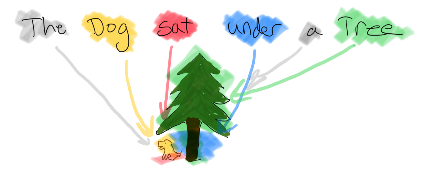
In this essay, I explain the motivation behind attention mechanisms, how attention works, and the details of two common types of attention mechanisms. This is a good starting point if you already understand how neural networks work, but don’t yet understand attention mechanisms.
What is attention?
Attention mechanisms are components in some neural networks that are inspired by human attention. When a human pays attention to something, the object of their attention is emphasized and all other things in the human’s field-of-view are de-emphasized. The result of “paying attention” is a representation of the object in their mind.
Attention mechanisms in neural networks behave analagously.
The “object” of attention is called the query. For example, the query could be a word embedding. The “field of view” of an attention mechanism is called the input or the input features. For example, the input features could be pixels in an image or a sentence of word embeddings.
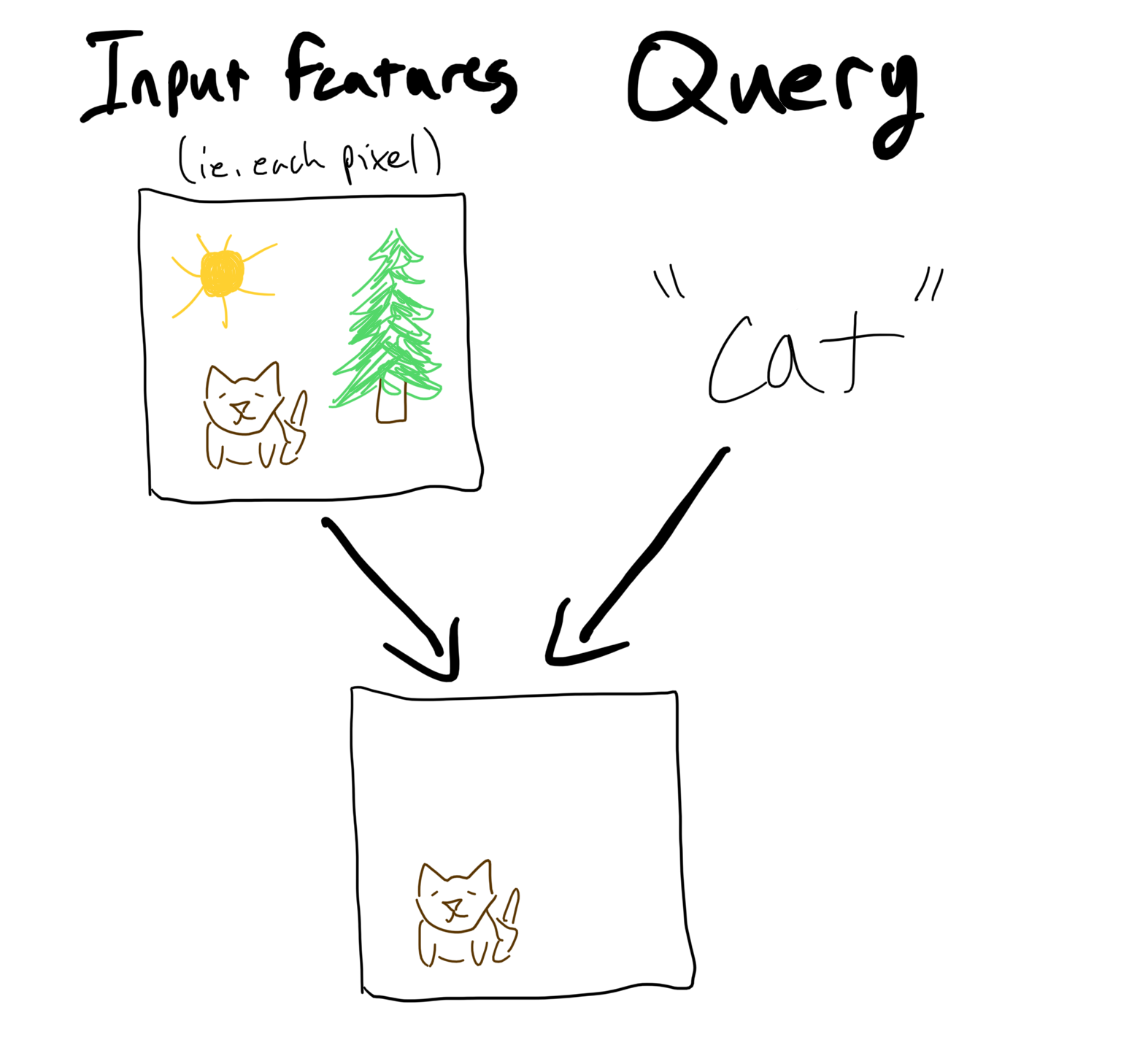
Attention mechanisms output a vector representation of importance-weighted parts of the input. This vector is called the context.
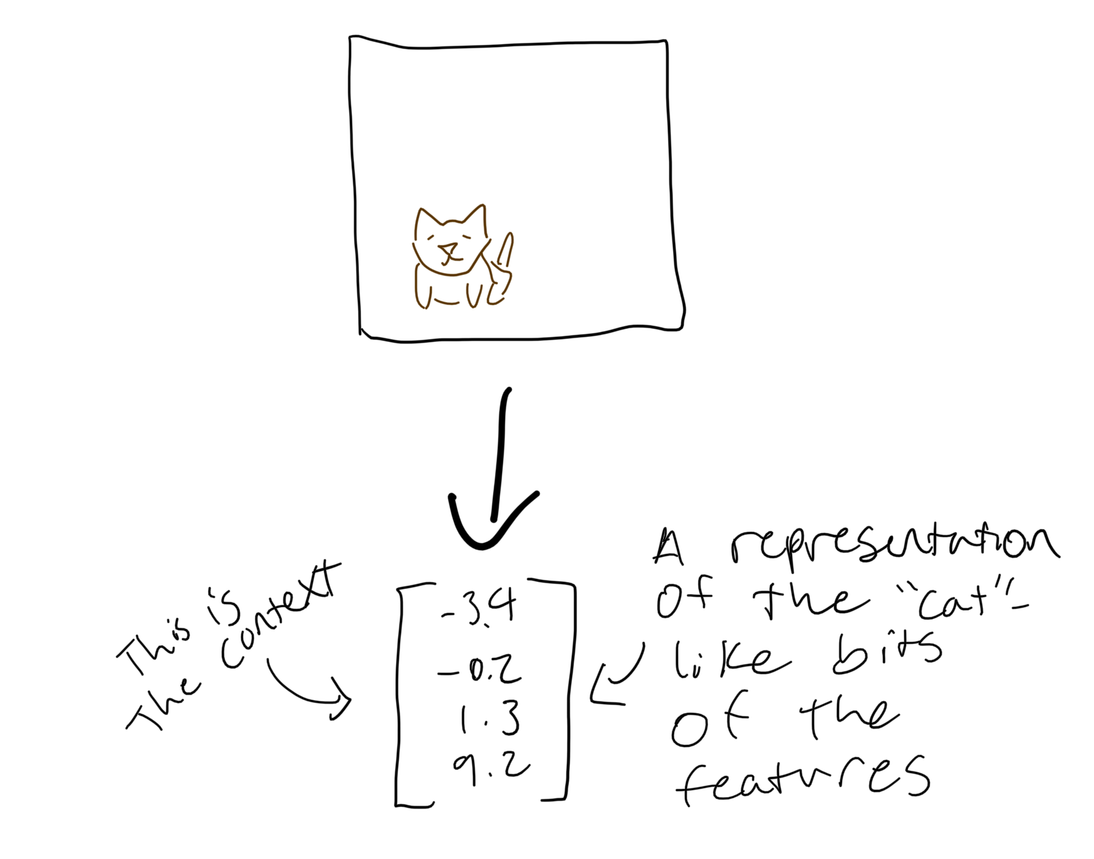
The name “context” comes from an early application of attention: providing a wider context for encoder-decoder RNNs. The inputs to an RNN are usually just the output of the previous RNN stage. This makes learning relationships across many steps more difficult, because you have to propagate the loss through many components. Since the context provides a relevance-weighted summary of the entire input, it provides a short path between any input feature and any output of the decoder RNN.
The four steps of attention mechanisms
There are different types of attention mechanisms, but all involve four steps:
- Create keys & values from the input: For each feature of the input, create a key and value.
- Score: For each key, score its relevance to the query. The scores are called attention scores.
- Align: Adjust the attention scores relative to each other. The adjusted scores are called the attention weights.
- Weight: Use the attention weights to weight and aggregate the values. The weighted and aggregated values is the context.
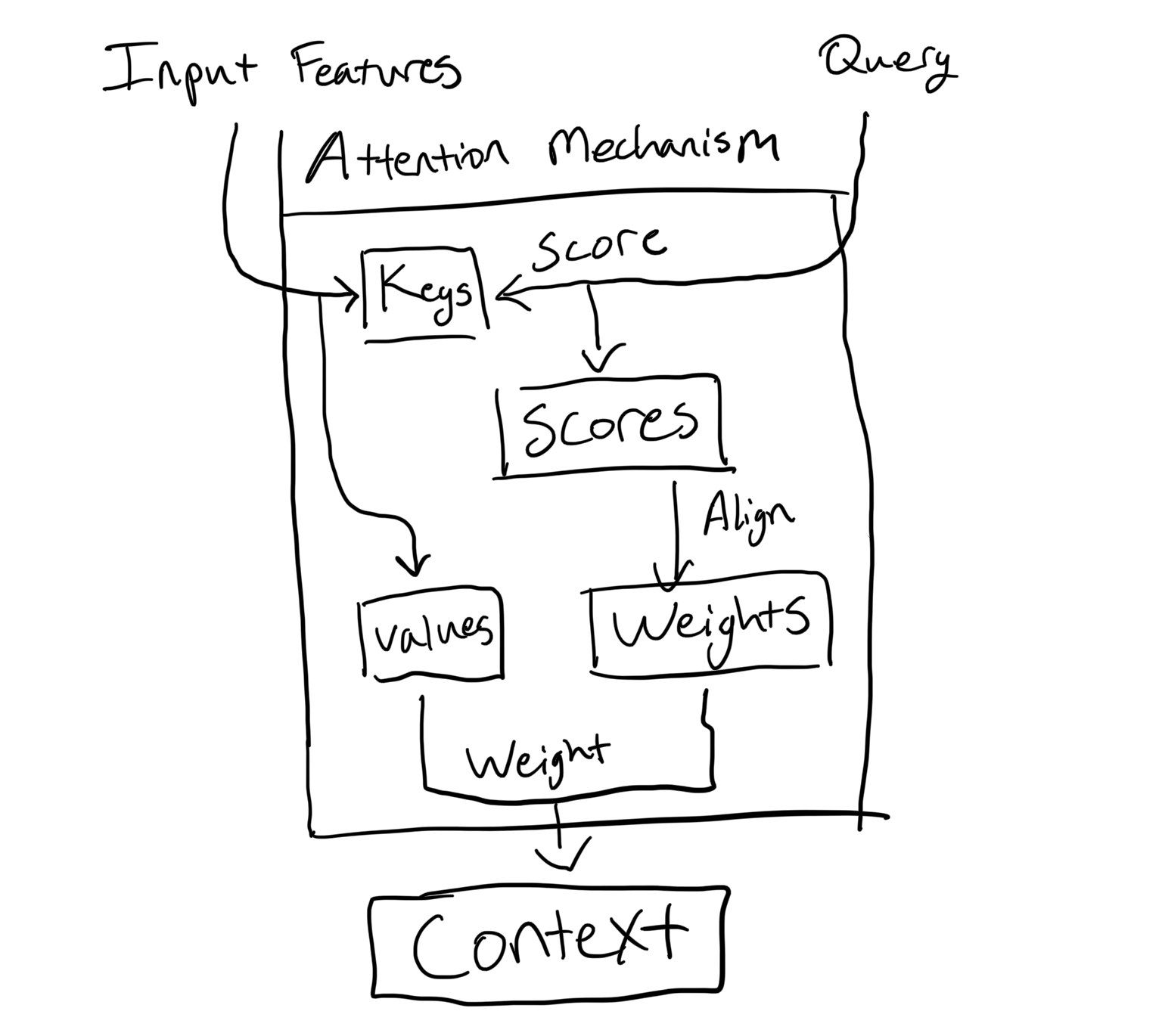
Let’s walk through each step.
Step 1: Create keys & values
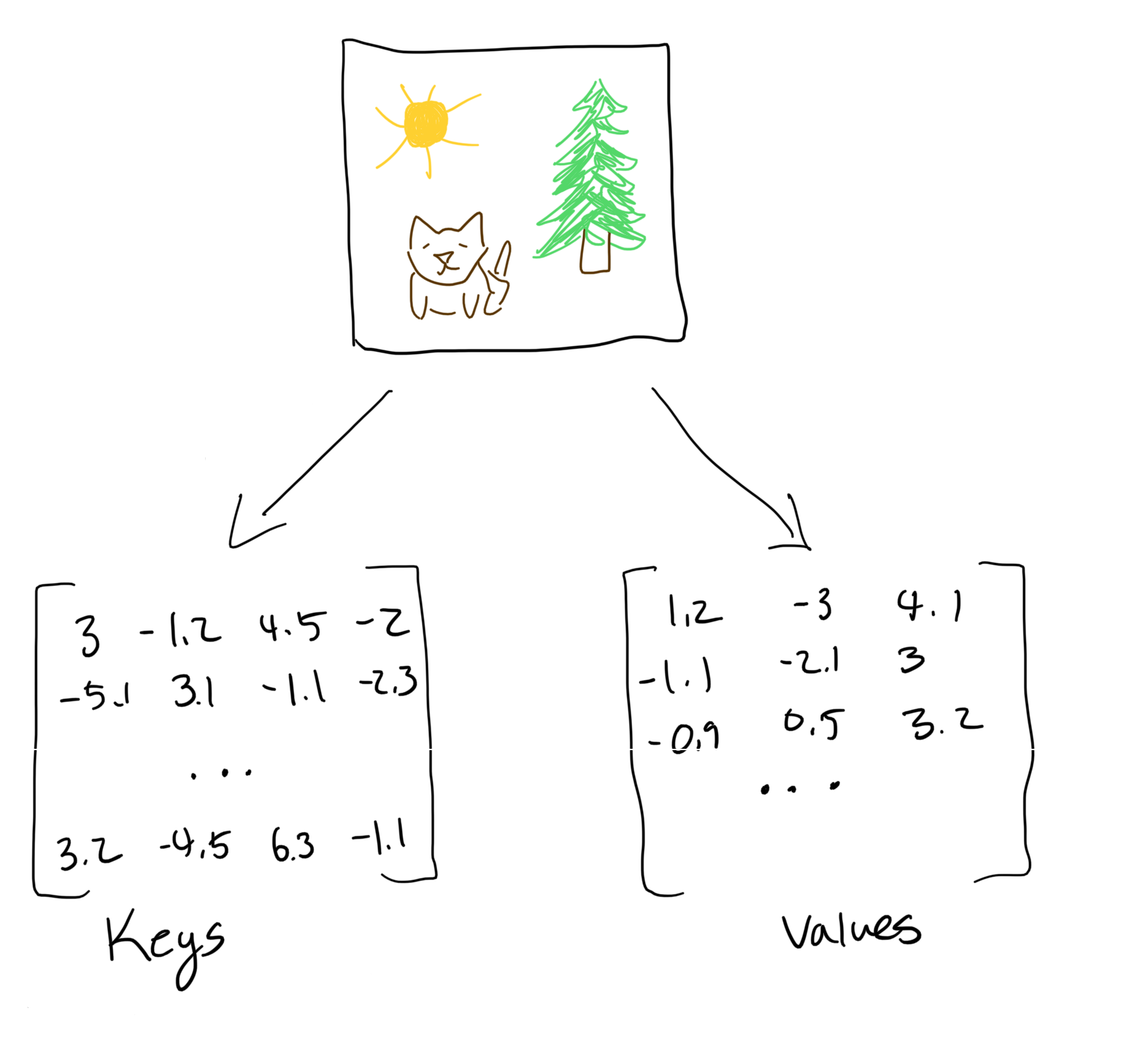
Some attention mechanisms create two separate representations of the input features, called keys and values.
It can be useful to separate “how to match relevance” and “how to provide useful context”.
Score
Now that we have the keys, we score how “relevant” each key is to the query. These are called attention scores.
Different types of attention mechanisms create attention scores differently. For example, you could use the dot product between the keys and the query.
Align
The scores present a problem: if all the scores are high, then everything in the input is “important”. If everything is important, there’s nothing to “focus” on. Likewise, if nothing is “important”, there’s nothing to focus on.
Therefore, we need adjust the scores relative to each other, so these two situations are equivalent. Usually the softmax function is used to adjust the scores relative to each other.
The adjusted scores are called the attention weights.
Weight
Now we use the attention weights to “focus” on the important parts of the input. We do this by multiplying each attention weight with its corresponding value (remember: we created the values in the first step).
This will give us the weighted values. Now, we need to aggregate them into a “context”. A common way to aggregate the weighted values is to add them together.
And voila! We have the context vector.
Example
To understand the steps, let us walk through an example. In the example, we’ll find the relevance of an English word (“dog”) to a French sentence (“le chien a mangé un biscuit”).
In this example, “dog” is the query and “le chien a mangé un biscuit” is the input.
Here is the query. We’re using a word embedding.
| dog |
|---|
| -4.3 |
| -1.2 |
| -3.2 |
Here are the input features. We’re using word embeddings for these too.
| le | chien | a | mangé | un | biscuit |
|---|---|---|---|---|---|
| 0.1 | 0.3 | -4.3 | 1.1 | 2.2 | 0.1 |
| -2.1 | -2.1 | -1.2 | 2.4 | 0.2 | 3.3 |
| -0.3 | -0.5 | -1.1 | 2.3 | 3.1 | 0.3 |
Create keys & values
The first step is to split the input features into keys and values.
A common method for finding the keys and values is via matrix multiplication with a learnable key parameter matrix and a learnable value parameter matrix.
To get the keys, we multiply each input feature by a weight matrix. In this example, the key parameter matrix is 2x3, which yields a 2x6 key matrix. The keys would look something like this:
| le | chien | a | mangé | un | biscuit |
|---|---|---|---|---|---|
| 0.1 | 0.3 | -4.3 | 1.1 | 2.2 | 0.1 |
| -2.1 | -2.1 | -1.2 | 2.4 | 0.2 | 3.3 |
Each key is a learned representation of the associated word.
To get the values, we multiply each input feature by a different parameter matrix . In this example, the value parameter matrix is 4x3, which yields a 4x6 key matrix. The values would look something like this:
| le | chien | a | mangé | un | biscuit |
|---|---|---|---|---|---|
| 0.1 | 0.3 | -4.3 | 1.1 | 2.2 | 0.1 |
| -2.1 | -2.1 | -1.2 | 2.4 | 0.2 | 3.3 |
| -0.3 | -0.5 | -1.1 | 2.3 | 3.1 | 0.3 |
| -0.3 | -0.5 | -1.1 | 2.3 | 3.1 | 0.3 |
Score
We use the keys to create an “attention score” for each input feature. We do this by comparing each “key” to each “query”. Different types of attention mechanisms have different scoring algorithms. For this example, we’ll use the dot product between each key and value. This can be done in a single matrix multiplication between the keys and the queries.
| dog | |
| le | 0.3 |
| chien | -2.1 |
| a | 5.5 |
| mangé | -1.2 |
| un | 3.2 |
| biscuit | -0.5 |
Alignment
The attention scores represent the pairwise “score” between each key and each query. However, these don’t represent the relative scores.
The most common alignment algorithm is softmax. That’s what we’ll use here.
| dog | |
| le | 0.2 |
| chien | 0.6 |
| a | 0.08 |
| mangé | 0.07 |
| un | 0.03 |
| biscuit | 0.02 |
Weighting
Now that we have the attention weights, we calculate the context.
Remember: the context is just a summary of the input, weighted by importance.
So, we just apply each attention weight to its corresponding value.
| le | chien | a | mangé | un | biscuit |
|---|---|---|---|---|---|
| 0.1 | 0.3 | -4.3 | 1.1 | 2.2 | 0.1 |
| -2.1 | -2.1 | -1.2 | 2.4 | 0.2 | 3.3 |
| -0.3 | -0.5 | -1.1 | 2.3 | 3.1 | 0.3 |
| -0.3 | -0.5 | -1.1 | 2.3 | 3.1 | 0.3 |
But this isn’t a vector: we need to summarize it into a learned representation.
For this example, we’ll just sum columns together to create the final context vector.
| Context |
|---|
| 0.1 |
| -2.1 |
| -0.3 |
| -0.3 |
And there we have it! We used attention to create a vector representation of the input.
Types of Attention
There are different types of attention mechanisms. Two common types of attention are additive attention (aka Bahdanau attention) and dot product attention.
Additive attention
Additive attention was introduced to help encoder-decoder RNNs translate text (Neural Machine Translation by Jointly Learning to Align and Translate by Bahdanau et al).
The input features are the “input” sentence. For example, if you’re translating French to English, the input is the French sentence.
Step 1: Create keys & values
In the original paper, the additive attention mechanism used the same thing for the keys and the values. Specifically, it used the hidden states of the encoder.
Step 2: Score
Additive attention calculates the attention score by using a mini neural net.
The attention neural net takes elements from both collections as input, and gives an unnormalized score.

It’s called “additive” attention, because of how the attention score is created. Specifically, the keys and the queries “combined” via addition (after applying matmul with parameters)
Step 3: Align
Now, we have the attention scores. To get the attention weights, just apply softmax to the scores.
Step 5: Weight
Apply each weight to its corresponding value. For additive attention, the values are the hidden states of the encoder.
Now, to get the context, we just sum the weighted values.
And there we go! We’ve calculated the context vector.
Here’s a worked example:
def score(keys, query):
	return v @ tanh(np.matmul(key_parameters, keys) + np.matmul(query_parameters, query))

def align(attention_scores):
	return softmax(attention_scores)

def weight(attention_weights, values):
	return attention_weights @ values

def additive_attention(input, query):
	keys = input
	values = input
	attention_scores = score(keys, query)
	attention_weights = align(attention_scores)
	return weight(attention_weights, values)
Scaled dot product attention
Scaled dot product attention was introduced in the 2017 paper Attention is all you need by Vaswani et al. It’s used in the massively popular Transformer neural network architecture.
Step 1: Create keys & values
Create keys by matrix multiplying learnable parameter matrices with the input features, just as in the earlier example. We create values in the same way.
Step 2: Score
Scaled dot-product attention calculates the attention score in two steps:
- Calculate the unscaled attention score by taking the dot product between the key and the query.
- Calculate the attention score by dividing the unscaled attention score by the square root of the number of dimensions in the key vector.
The dot product calculates the overlap between two vectors. If the key and query are pointing in totally different directions, their overlap will be low and therefore the score will be low. Likewise, if the key and query point in very similar directions, their score will be high and therefore the score will be high.
The unscaled attention score might be okay to use by itself, but there’s a technical detail which could cause a problem: if the keys are very high dimensional, the unscaled attention scores could get very large. If the scores are very large, the gradients could be very large, which could make the training process more challenging.
To prevent the attention scores from getting larger with different key sizes, we just divide the unscaled attention scores by the square root of the dimensionality of the keys.
Step 3: Align
To calculate the attention weights, we use the softmax function on the attention scores.
Step 4: Weight
Apply the attention weights to the values, by multiplying them together. This deemphasizes irrelevant values and emphasizes relevant values.
A worked example…
# For the toy example, create some random input.
collection_a = np.random.randn(4)
collection_b = np.random.randn(6)

# Initialize the attention mechanism’s weights.
key_weight_matrix = np.random.randn(4, 5)
query_weight_matrix = np.random.randn(6, 5)
value_weight_matrix = np.random.randn(6, 5)

# Calculate the keys, and queries.
queries = np.matmul(collection_a, query_weight_matrix)
keys = np.matmul(collection_b, key_weight_matrix)

# Find how “related” are the keys and queries.
scores = np.matmul(queries, keys)

# Normalize the scores to find the attention weights.
attention_weights = softmax(scores, dim=1)

# Use the scores to find the output.
values = np.matmul(collection_b, value_weight_matrix)
output = attention_weights @ values
Recap
- Attention mechanisms are trainable components of some neural networks
- Attention mechanisms output a “context”. The context is a vector representation that encodes the “relevant” parts of the input.
- There are different types of attention mechanisms, such as additive attention and dot-product attention
- Additive attention uses a small neural network to calculate the attention score.
- Scaled dot-product attention uses the dot product to calculate the unscaled attention scores. It divides the unscaled attention scores by the square root of the key dimensionality, to prevent the scores from getting too big.
Relevant sources
- Neural Machine Translation by Jointly Learning to Align and Translate
- Paper from 2015.
- Introduces additive attention for translation
- Uses a mini FFNN to compute attention score
- Luong Attention Paper
- Attention is All You Need
- Introduces scaled dot-product attention
- A General Survey on Attention Mechanisms in Deep Learning
- A helpful overview of attention and attention mechanisms